Vapnik–Chervonenkis Dimension and Polynomial Classifiers
In this post we will explore a rather unusual sort of binary classifier: the generalized polynomial classifiers. Our primary goal is to determine analytical bounds on the VC-dimension of this family of classifiers, giving some indication as to their potential expressive power.
Generalized Polynomial Classifiers
A generalized polynomial classifier is a binary classifier of the form
![\[H(x) = \begin{cases}+1 &\text{if } p(x) > 0 \\-1 &\text{if } p(x) \le 0\end{cases}\]](https://russ-stuff.com/wp-content/ql-cache/quicklatex.com-4af024ef4deb37735971f678e2e66a53_l3.png "Rendered by QuickLaTeX.com")
for multi-variate polynomials
 of degree
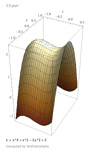
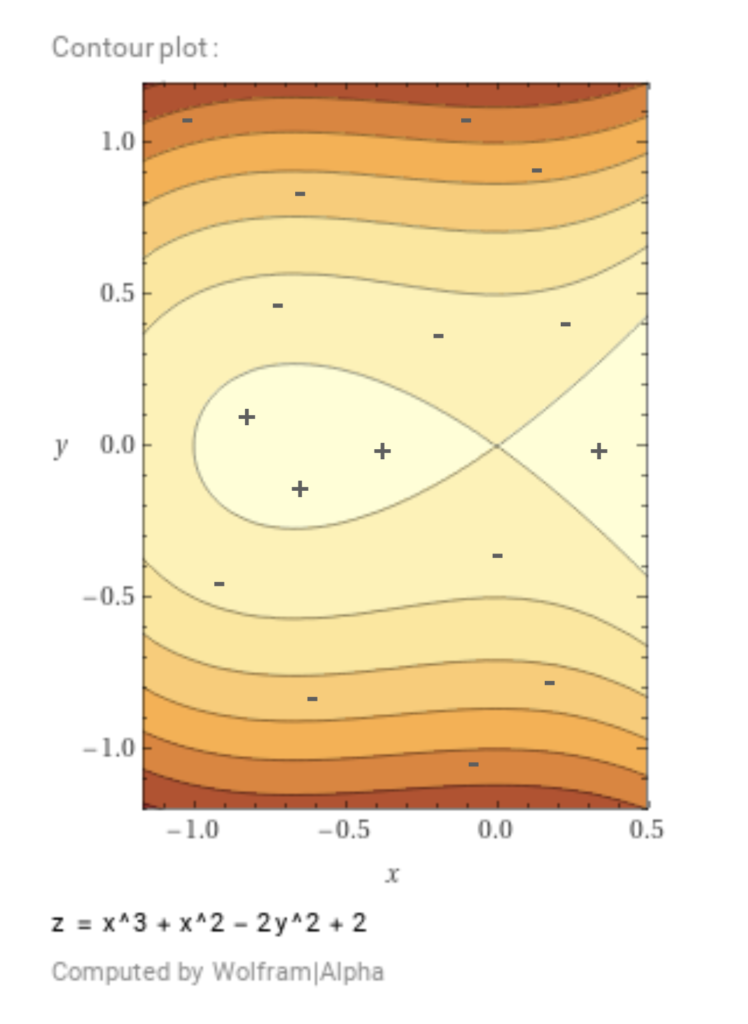
  . While polynomials are often used for regression tasks, here we investigate their use in classification. For example, the polynomial
  gives a highly non-linear decision boundary:
Depending on the dimension of the feature space and the value of  , these classifiers resemble some more familiar models:
- When our feature space is
 and is arbitrary, the polynomial is a conventional polynomial of a single real variable:
In this case, finding![\[p(x) = a_0 + a_1x + \cdots a_{d}x^d\]](https://russ-stuff.com/wp-content/ql-cache/quicklatex.com-1537d661089a8c17fba6b7e41fcdf34b_l3.png "Rendered by QuickLaTeX.com")
 is a polynomial interpolation task, and
  partitions the real line into positive and negative regions delineated by the roots of .
 - When our feature space is
 and is arbitrary, the polynomial is a polynomial of two variables:
In this case, finding![\[p(x, y) = a_0 + a_1x + a_2y + a_3x^2 + a_4y^2 + a_5xy + a_6x^3 + a_7x^2y + \cdots\]](https://russ-stuff.com/wp-content/ql-cache/quicklatex.com-124683c064dd0d1533052dcbb39aef4a_l3.png "Rendered by QuickLaTeX.com") is a surface-fitting task, and the resulting partitions the plane into regions delineated by the iso-contours
is a surface-fitting task, and the resulting partitions the plane into regions delineated by the iso-contours  .
. - When our feature space is
 and
and  , we have a not-uncommon quadratic form:
expressed in terms of conventional matrix-vector products.![\[p(x) = A_0 + A_1x + x^\T A_2 x\]](https://russ-stuff.com/wp-content/ql-cache/quicklatex.com-d30fc7f4b4b607dbcce1f91cff6d9ead_l3.png "Rendered by QuickLaTeX.com")
- When our feature space is and is arbitrary, we have the most general form
where![\[p(x) = A_0 + A_1x + A_2x^2 + \cdots + A_dx^d\]](https://russ-stuff.com/wp-content/ql-cache/quicklatex.com-eeb6a0583750be75b2fff3d76582e4ab_l3.png "Rendered by QuickLaTeX.com")
 is a tensor1 of rank
  and
and  denotes the -mode product:
Hence,![\[A_kx^k = \sum_{i_1, \cdots, i_k} A_k[i_1, \cdots, i_k]x[i_1] \cdots x[i_k]\]](https://russ-stuff.com/wp-content/ql-cache/quicklatex.com-4ca59f62af9df1d926b73c127417e42c_l3.png "Rendered by QuickLaTeX.com")
 is a scalar,
  a vector,
  a matrix, etc.
For example, over  with , we have the general form:
![\[p(x) = A_0 + \begin{pmatrix}A_1[0] \\ A_1[1] \\ A_1[2]\end{pmatrix}\begin{pmatrix}x \\ y \\ z\end{pmatrix} + \begin{pmatrix} A_2[0, 0] & A_2[0, 1] & A_2[0, 2] \\ A_2[1, 0] & A_2[1, 1] & A_2[1, 2] \\ A_2[2, 0] & A_2[2, 1] & A_2[2, 2] \\ \end{pmatrix}\begin{pmatrix}x \\ y \\ z\end{pmatrix}\]](https://russ-stuff.com/wp-content/ql-cache/quicklatex.com-9e17867f2a60ff43eb97ec1e68937d5b_l3.png "Rendered by QuickLaTeX.com")
A GPC can be viewed as a generalization of an SVM with a polynomial kernel. The number of coefficients (and hence the number of potentially trainable parameters) is given by:
![\[\sum_{k=0}^d \binom{n+k-1}{k} = \binom{d+n}{d} = O\left(n^d\right)\]](https://russ-stuff.com/wp-content/ql-cache/quicklatex.com-54832c71a07bd390b869aadcc97e8748_l3.png "Rendered by QuickLaTeX.com")
Note that our chosen representation has some constant redundancy factor, which we can eliminate by stipulating WLOG that be upper-triangular. This exponential growth in the number of parameters indicates that the expressive power of a GPC is likely quite high. However, it also indicates that training may be impractical, and that overfitting may be a serious issue.
We will use the notation  to denote the family of polynomial classifiers over
  of dimension .
Note that since we are using a regression tool for classification, we need to develop a continuous encoding for discrete labels. We use the obvious choice:
![\[(x, +) \mapsto (x, +1)\]](https://russ-stuff.com/wp-content/ql-cache/quicklatex.com-e47f8be751750d4746ab0a35d567351e_l3.png "Rendered by QuickLaTeX.com")
![\[(x, -) \mapsto (x, -1)\]](https://russ-stuff.com/wp-content/ql-cache/quicklatex.com-80efbdbfb6da878b52283738d4ab4ee5_l3.png "Rendered by QuickLaTeX.com")
VC Dimension
VC-dimension, short for Vapnik–Chervonenkis Dimension, is a measure of the expressive power of a family of classifiers. It is defined as the size of the largest set of points that can be correctly classified (by a member of the family in question) for any assignment of binary labels. We sometimes say that the point set is “shattered” by the classifier in this case.
For example, consider a 2-dimensional feature space and the family of linear classifiers (i.e. classifiers whose decision boundaries are lines). This conventional family of classifiers is effectively just  . Clearly, for any set of three points and any assignment of +/- labels, the data is linearly separable. However, no arrangements of four points can be shattered. There are two cases to consider:
- All four points are contained in the convex hull. Assign labels such that only opposite points have the same label (as in Figure 1). The resulting arrangement is not linearly-separable.
- Only three points are contained in the convex hull. In this case, one point is necessarily contained in a triangle formed by the other three. Assign the three hull points + and the one internal point -. The resulting arrangement is not linearly-separable.
This argument shows that the VC dimension of the family of 2D linear classifiers is  .
.
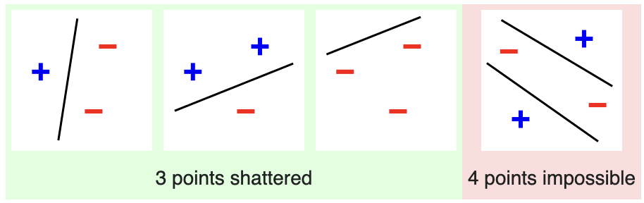
 and (case (2) omitted). (Image Credit)
As another point of reference, the VC-dimension of a neural network using the sigmoid non-linearity is known to be quadratic in the number of trainable parameters. Specifically, the VC-dimension is  where
where  and
and  represent the edges and vertices in the network’s computation graph.
We will use the notation  to denote the VC-dimension of a family of classifiers.
Theoretical Analysis of GPCs
First, an easy result on the monotonicty of the VC-dimension.
Theorem 1. Let  and
and  . Then,
Proof. The result follows immediately from the fact that  .
.
In the special case of polynomial classifiers over  , the VC dimension is relatively straightforward to compute.
Theorem 2. 
Proof. Since a polynomial of degree can have at most roots, it can only partition the real line into at most  regions of alternating sign. Consequently, a set of
  sorted points with alternating labels:
![\[\{(x_1, +1), (x_2, -1), (x_3, +1), \cdots, (x_{d+2}, +1)\}\]](https://russ-stuff.com/wp-content/ql-cache/quicklatex.com-d9fe148e487cc8d89be69cbb7212ce0d_l3.png "Rendered by QuickLaTeX.com")
cannot be correctly classified by any member of  . Thus, .
Theorem 3. 
Proof. For any set of points, there exists a polynomial (in fact, exactly one polynomial) of degree that interpolates the points. Thus, any given labelled points  can be classified exactly regardless of labelling by constructing the interpolating polynomial (by lagrange interpolation, for example). Thus,
  .
.
The prior two results show that  . We can also derive some explicit values for linear polynomials (i.e. hyperplane decision boundaries).
Theorem 4. 
Proof. Take  points from as the vertices of a simplex as follows:

We claim that these points can be correctly classified for any label assignment. Let  denote the indices of the points that are assigned a + label. We construct a linear polynomial such that
![\[p(x_i) = \begin{cases}1 &\text{if } i \in I \\0 &\text{if } i \notin I \\\end{cases}\]](https://russ-stuff.com/wp-content/ql-cache/quicklatex.com-59078bb7aaec843918375fab87f57077_l3.png "Rendered by QuickLaTeX.com")
giving us exactly the desired classification. There are two cases:
- If
 , then we take
 ![p(x) = 1 - \sum_{j \notin I} x[j]](https://russ-stuff.com/wp-content/ql-cache/quicklatex.com-a220f4c321f364a3fee05cce7c3473d5_l3.png "Rendered by QuickLaTeX.com")
- If
 , then we take
 ![p(x) = \sum_{i \in I} x[i]](https://russ-stuff.com/wp-content/ql-cache/quicklatex.com-7096c3fc61dbecdf5a11a3c7e0c77eb7_l3.png "Rendered by QuickLaTeX.com")
It is easy to see that gives the correct activation in both cases. Thus, we have shown that there exists a set of points that can always be shattered.
We now present the main result, an asymptotic lower bound for arbitrary dimension and degree. We begin with the special case of  and then show that the approach generalizes.
Theorem 5. 
Proof. Consider a set of  points in the plane arranged as the vertices of an
  integer lattice (with
  to be determined later). In particular, take
  . Assign +1/-1 values to the points arbitrarily. Now, consider each row of the lattice independently, and fit a 1D interpolating polynomial
  to row
  . We wish to construct a 2D polynomial out of the
  ‘s by somehow interpolating between them. To do this, define the following family of “selector” polynomials. Let
  be the 1D polynomial that interpolates:
![\[(0, 0), (1, 0), \cdots, (i, 1), \cdots, (N-1, 0)\]](https://russ-stuff.com/wp-content/ql-cache/quicklatex.com-996eeeddc53f84281404bfb686bd8542_l3.png "Rendered by QuickLaTeX.com")
Informally, “selects” point while rejecting all others. We can now define our 2D polynomial as follows.
![\[p(x, y) = \sum_{i=0}^{N-1} p_i(x) \cdot \phi_i(y)\]](https://russ-stuff.com/wp-content/ql-cache/quicklatex.com-e6f055ab4d89f44b4be4943fb8f68d6a_l3.png "Rendered by QuickLaTeX.com")
We can see that  selects the appropriate row and gets the appropriate value from that row, thus correctly interpolating the full dataset. Since and
  are both of degree
  , the resulting is of degree
  . We require this quantity to be less than , so we take
  . We have thus demonstrated a way to correctly classify
  2D points using a 2D polynomial of degree regardless of labelling. Therefore, .
Theorem 6. 
Proof. The proof of Theorem 5 generalizes nicely. We will construct an arrangement of points in that can be shattered. First, consider the largest arrangement of points in  that can be shattered by a polynomial of degree ; that is, an arrangement of
  many points. Take copies of this arrangement and stack them along the
  th dimension (in 3D, this looks like slices stacked vertically). Assign +1/-1 values to the points arbitrarily. For each slice , take as the
  -D polynomial that correctly classifies the points. We now define our full -D polynomial:
![\[p(x) = \sum_{i=0}^{N-1} p_i(x[0], x[1], \cdots, x[n-2]) \cdot \phi_i(x[n-1])\]](https://russ-stuff.com/wp-content/ql-cache/quicklatex.com-959c64c023f4c7eb38c5a05954cd3ca8_l3.png "Rendered by QuickLaTeX.com")
We can see that selects the appropriate slice and gets the appropriate value from that slice, thus correctly interpolating the full dataset. Since and are both of degree , the resulting is of degree . We require this quantity to be less than , so we take . We have thus demonstrated a way to correctly classify  many -D points using a -D polynomial of degree regardless of labelling. Therefore,

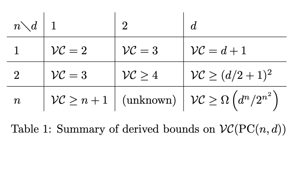
We can solve this recurrence with the base case established by Theorem 5 to obtain the main result:

It is exciting to see that the expressive power of polynomial classifiers exhibits (at least) exponential asymptotic growth. However, the curse of dimensionality is strong, with the doubly exponential constant term dependent on .
The results are summarized in the following table
Training GPCs
One immediate way to train a multivariate polynomial classifier is to treat the higher-order terms as the output of a lifting kernel and solve the resulting linear system:

This matrix is a the multivariate analog of the Vandermonde matrix for ordinary polynomial interpolation and is of size  . Solving this system (in the least-squares sense) via SVD requires at least
  operations. If the number of parameters is fixed for a given classifier to-be-trained, this approach is effectively quadratic in the number of training points.
Another approach is to learn the weights gradually via gradient descent. We can pass the output of the polynomial through a sigmoid function ![\sigma: (-\infty, \infty) \to [0, 1]](https://russ-stuff.com/wp-content/ql-cache/quicklatex.com-4c5001e494befd2b613407fc1168703b_l3.png "Rendered by QuickLaTeX.com") and then define a cross-entropy loss function. However, this approach may incentivize learning large coefficients so some regulatory terms may be needed in the loss function, or possibly some other kind of non-linear transform on top of the polynomial may be required. Implementing this approach is an avenue for future work.
and then define a cross-entropy loss function. However, this approach may incentivize learning large coefficients so some regulatory terms may be needed in the loss function, or possibly some other kind of non-linear transform on top of the polynomial may be required. Implementing this approach is an avenue for future work.
Conclusion
In this post we investigated the VC-Dimension of the family of generalized polynomial classifiers for binary classification over multi-dimensional feature space. Exact values are computed for low dimension and low degree, and asymptotic bounds are derived for the general form. The quadratic dependence on dimension indicates that the approach may only be suitable for lower-dimension feature spaces in which the degree of the polynomial is much higher than the number of features. However, in these settings, they may prove comparable to neural networks as a universal function approximator.
Methods for training GPC’s were briefly discussed, but more work is required to see if they are really very practical to use (my guess is probably not 😛). Cheers!