The Bayes Filter for Robotic State Estimation

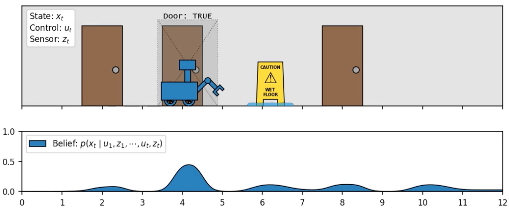
Posted on October 17, 2023January 25, 2024 by Russell Schwartz

Figure 1: Bayes Filter state estimation of a mobile robot in an indoor environment.
Sensor measurements $z$ and control inputs $u$ are combined over time to form an
estimate of the robot’s current state $x$ (in this case, it’s location in the hallway).

Introduction¹

State estimation is a fundamental challenge in robotics. Before a robot can take an action, it has to have some understanding of the environment it inhabits, as well as its relationship to that environment. The state can include any potential unknown quantity, including things like the robot’s position and velocity, the angle of it’s joints, the temperature in the room, the positions of other objects, or even the onboard sensors’ calibration parameters. We usually represent the state numerically as a vector $x \in \mathbb{R}^d$ . For instance, a robot vacuum cleaner might have state vector

$\begin{bmatrix}x \\ y \\ \theta \\ bat \\ vac\end{bmatrix} = \begin{bmatrix}12.5 \\ -3.2 \\ 0.7 \\ 0.98 \\ 0\end{bmatrix}$

where $x, y, \theta$ represent position/orientation, $bat \in [0, 1]$ represents battery level, and $vac \in \{0, 1\}$ represents whether the vacuum is on or not. The main way we obtain a state estimate is by making measurements of the environment. For instance, our robot vacuum might be equipped with wheel rotation sensors, a front-mounted camera, and a battery voltage sensor.

The challenge is that sensors are imperfect and often tell incorrect or contradictory stories. In almost all cases, the values a sensor reports will be corrupted by some amount of error or noise. The hope is that by taking many measurements over time, the errors in our readings will cancel out, allowing us to obtain an accurate estimate of the true state. This process of combining noisy measurements over time is called filtering.

Perhaps the first filtering method that comes to mind is the humble moving average, in which we simply take the mean of past measurements to obtain our estimate (possibly by restricting our attention to a recent window of the past, or alternatively by weighting measurements by some time-dependent discount factor). This is frequently effective in smoothing the signal and reducing error, as in the example pictured here.

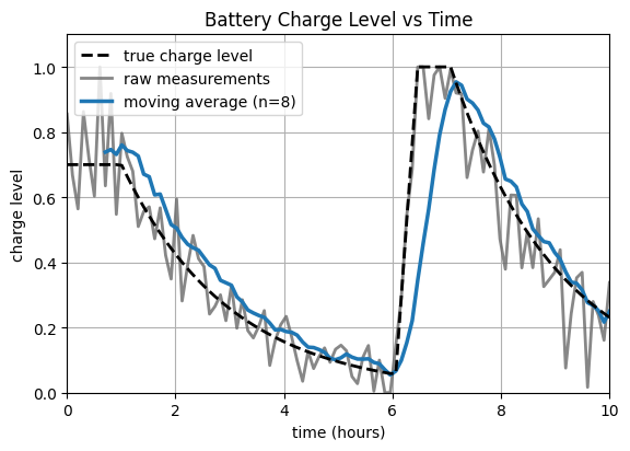
However, a simple moving average has several deficiencies. First, it induces a significant temporal lag in our state estimate, which may be undesirable. Second, it provides no immediate mechanism for us to combine evidence from different sensors. Third, it does not explicitly model the amount of uncertainty in our state estimates. This last point is especially important.

It is not sufficient to track only our best guess of the current state. We must also track our uncertainty in this guess. In our battery example, 10 voltage measurements with a (confidence-inspiring) 1% spread should result in less uncertainty in our reported state estimate than, say, 3 measurements with a (not-so-inspiring) 20% spread. We should also be able to incorporate external information about the quality of a sensor into our reasoning.

The Bayes Filter formalizes these ideas and provides a mathematical framework for representing our state estimate while modeling uncertainty in such a way that allows us to incorporate new measurements from multiple different sensors. Moreover, it does this optimally. The core idea is that we model our belief of the current state as a probability distribution over the domain of possible state values.

In this post we will derive the filter update rules and show some examples of it running in simulation, but first we must review some classical probability.

Causal vs Diagnostic Reasoning

Suppose we are designing a weather station that can tell us whether it is currently raining or not. To do this, we deploy a sensor which measures electric conductivity in the soil and reports a value $z \in \{\mathsf{wet}, \mathsf{dry}\}$ . Let $x \in \{\mathsf{rainy}, \mathsf{clear}\}$ represent the current state of the weather. Presumably, the random variables $x$ and $z$ are closely related, allowing us to use information about one to gain insight into the other. There are two different ways in which we can quantity this relationship:

$P(x = \mathsf{rainy} \mid z = \mathsf{wet})$ : the probability that it is rainy, given that we observe wet soil
$P(z = \mathsf{wet} \mid x = \mathsf{rainy})$ : the probability that we observe wet soil, given that it is rainy

The first of these, $P(\mathsf{rainy} \mid \mathsf{wet})$ , can be thought of as diagnostic knowledge.² The second, $P(\mathsf{wet} \mid \mathsf{rainy})$ , can be thought of as causal knowledge. Even though diagnostic information is usually what we really care about, often times, causal knowledge is easier to obtain. For instance, we can run some experiments to determine that the soil sensor reports $\mathsf{wet}$ 90% of the time when it’s raining, and $\mathsf{dry}$ 80% of the time when it’s clear. That is, $P(\mathsf{wet} \mid \mathsf{rainy}) = 0.9$ and $P(\mathsf{dry} \mid \mathsf{clear}) = 0.8$ .

The question becomes, how do we convert the causal knowledge that we do have into useful diagnostic knowledge? The answer is Bayes’ Rule:

$P(\mathsf{rainy} \mid \mathsf{wet}) = P(\mathsf{wet} \mid \mathsf{rainy}) \frac{P(\mathsf{rainy})}{P(\mathsf{wet})}$

Bayes’ Rule tells us that the conditional probabilities are related by the ratio of the unconditioned probabilities. These values are usually not hard to obtain. For the state $x$ , we can use historical data to determine that $P(\mathsf{rainy}) = 0.25$ and $P(\mathsf{clear}) = 0.75$ . For the measurement $z$ , we can use the law of total probability:

$P(\mathsf{wet}) = P(\mathsf{wet} \mid \mathsf{rainy})P(\mathsf{rainy}) + P(\mathsf{wet} \mid \mathsf{clear})P(\mathsf{clear}) = 0.9 \times 0.25 + 0.2 \times 0.75 = 0.375$

Putting it all together, we finally get the diagnostic information we care about:

$P(\mathsf{rainy} \mid \mathsf{wet}) = 0.9 \times \frac{0.25}{0.375} = \mathbf{0.6}$

Now, if we observe wet soil, we can report to the users of our weather station that there is a 60% chance that it’s raining.³ Our initial belief before making the measurement is called the prior and our updated belief after incorporating the new information is called the posterior.

Combining Measurements

Suppose we obtain a second observation of wet soil 1 hour after the first. How can we integrate this new information into our estimated state? More generally, how can estimate $P(x \mid z_1, \cdots, z_n)$ ? To begin, we can apply Bayes’ Rule on the most recent measurement to try to separate it from all the measurements that came before:

$P(x \mid z_1 \cdots z_n) = \frac{P(z_n \mid x, z_1, \cdots, z_{n-1}) P(x \mid z_1 \cdots, z_{n-1})}{P(z_n \mid z_1, \cdots, z_{n-1})}$

Let’s take a closer look at $P(z_n \mid x, z_1, \cdots, z_{n-1})$ . If we are given the current state $x$ , then it seems like the old measurements $z_1, \cdots, z_{n-1}$ , which were made about a past state, are really sort of redundant. Indeed, measurements are independent of one another when conditioned on the state. This is what’s called the Markov Property:

$P(z_n \mid x, z_1, \cdots, z_{n-1}) = P(z_n \mid x)$

This allows us to simplify our computation considerably. In fact, we can apply Bayes’ Rule followed by the Markov Property repeatedly to fully expand the formula. For convenience, we absorb the normalization terms $1/P(z_n \mid z_1, \cdots, z_{n-1})$ into the constant $\eta$ .

$\begin{align*}P(x \mid z_1 \cdots z_n) &= \eta P(z_n \mid x, z_1, \cdots, z_{n-1}) P(x \mid z_1 \cdots, z_{n-1}) \\&= \eta P(z_n \mid x) P(x \mid z_1 \cdots, z_{n-1}) \\&= \eta P(z_n \mid x) P(z_{n-1} \mid x) P(x \mid z_1 \cdots, z_{n-2}) \\&= \eta P(z_n \mid x) P(z_{n-1} \mid x) P(z_{n-2} \mid x) P(x \mid z_1 \cdots, z_{n-3}) \\&= \cdots \\&= \eta \prod_{i=1}^n P(z_i \mid x) P(x)\end{align*}$

Exercise: Using the framework for combining measurements, compute $P(\mathsf{rainy} \mid \mathsf{wet}_1, \mathsf{wet}_2)$

▸ See Solution

We apply the multi-measurement Bayes’ Rule:

$\begin{align*}P(\mathsf{rainy} \mid \mathsf{wet}_1, \mathsf{wet}_2) &= \eta P(\mathsf{wet}_1 \mid \mathsf{rainy}) P(\mathsf{wet}_2 \mid \mathsf{rainy}) P(\mathsf{rainy}) \\&= \eta \times 0.9 \times 0.9 \times 0.25 \\&= 0.2025 \eta \\\quad \\P(\mathsf{clear} \mid \mathsf{wet}_1, \mathsf{wet}_2) &= \eta P(\mathsf{wet}_1 \mid \mathsf{clear}) P(\mathsf{wet}_2 \mid \mathsf{clear}) P(\mathsf{clear}) \\&= \eta \times 0.2 \times 0.2 \times 0.75 \\&= 0.0300 \eta\end{align*}$

and then normalize:

$\begin{align*}0.2025 \eta + 0.0300 \eta &= 1 \implies \eta = 4.30108 \\\quad \\\implies P(\mathsf{rainy} \mid \mathsf{wet}_1, \mathsf{wet}_2) &= 0.2025 \times 4.30108 \approx \mathbf{0.87} \\\implies P(\mathsf{clear} \mid \mathsf{wet}_1, \mathsf{wet}_2) &= 0.0300 \times 4.30108 \approx 0.13\end{align*}$

Representing Belief

If our state domain is discrete, as in the weather station example, we represent our belief about the current state by a Probability Mass Function (or PMF), which can be fully described by a finite set of values. If instead our state is continuous, as it so often is in robotics, we need to use a Probability Density Function (or PDF), which are generally more difficult to describe fully.

Let’s move our attention to the motivating example of a (continuous-state) localization problem.⁴ Suppose we have a robot traversing an indoor space. To keep things simple, let’s limit our environment to a single (one-dimensional) hallway. Our state consists of just one value: the robot’s location $x \in \mathbb{R}$ in meters.

Figure 3: Simplified 1D Localization Problem
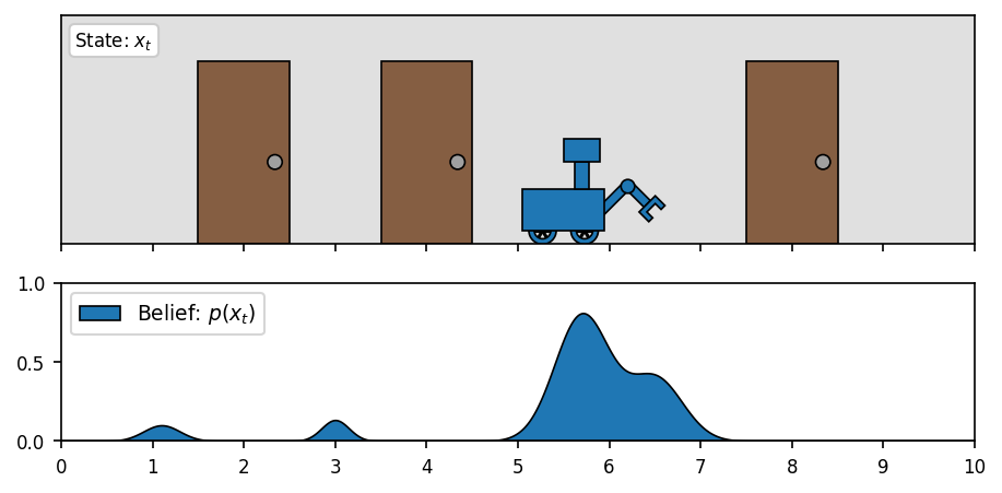
(belief is any arbitrary PDF over the domain)

There a number of ways to represent the belief PDF under-the-hood. Here, we use a histogram-based method that works by discretizing the domain and assigning some probability mass to each region. There are other ways, including particle-based methods and parametric methods. These give rise the to Particle Filter and Kalman Filter respectively, which we will discuss more later.

Measurement Models

Continuing with the localization example, let’s say our little robot is equipped with a camera that it can use to detect when it is in front of a door. Additionally, let’s say we have access to a map of the hallway which includes the true locations of all the doors: $\mathsf{doors} = \{2, 4, 8\}$ . The goal is to estimate our location with respect to this map.

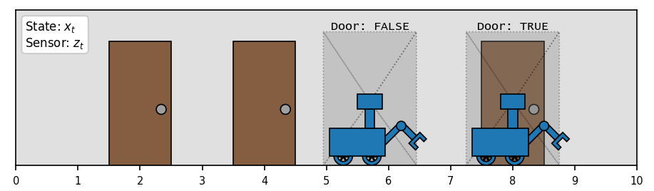
The first ingredient we will need to starting implementing the Bayes Filter is a Measurement Model: $P(z \mid x)$ , which specifies the expected behavior of our sensor under different states. We saw this before in the weather station example. In this case, our measurement model estimates the probability that the sensor reports seeing a door for every possible robot position $x$ . It might look something like this:

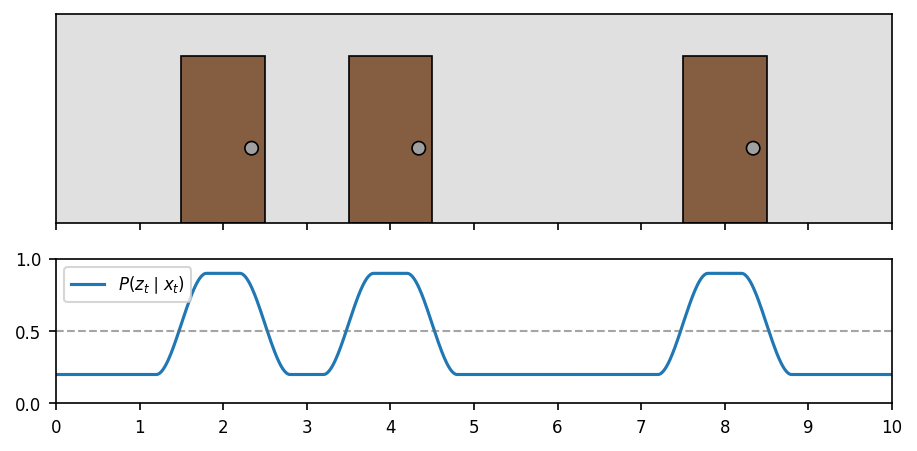
Figure 5: Door Detector Measurement Model

According to this (rather pessimistic) model, the sensor reports seeing a door 90% of the time when there actually is one in front of us, and 20% of the time when we’re really just looking at a wall. The model transitions smoothly between these probabilities when a door is only partially within our field of view.

The door-detector returns one of a finite set of possible measurements $z \in \{\mathsf{TRUE}, \mathsf{FALSE}\}$ , so the sensor model needs only to assign a scalar probability value to each possible measurement (i.e. a Probability Mass Function), for every state in our domain. Since this particular PMF can be uniquely described by a single value $P(z = \mathsf{TRUE})$ , we can visualize the sensor model as above. However, in general our sensors might return any of an infinite number of possible measurements. Common measurement spaces include $\mathbb{R}$ , $\mathbb{R}^m$ , and $\mathrm{SO}(3)$ . In these cases, the sensor model will have to define a full-fledged PDF over the space of possible measurements, for every state in our domain.

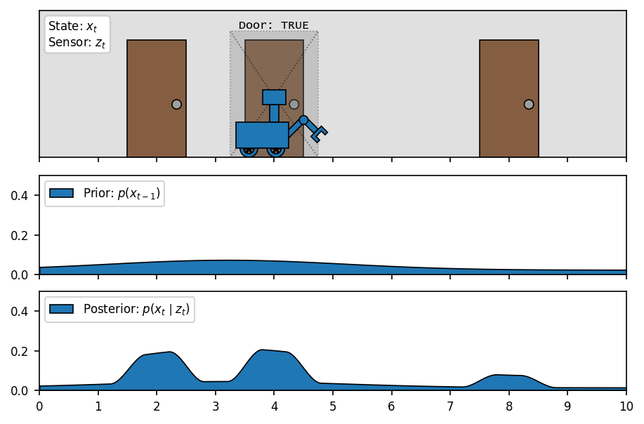
Figure 6: Measurement Model Example
(after observing the door, belief is updated)

From sensor modeling alone, we could implement our framework for combining evidence to accurately estimate whether the robot is in front of a door or not, but how can we tell which door? For that, we have to exploit our knowledge of the robot’s motion.

Action Models

The missing piece of the puzzle lies in the sequence of known actions (aka control inputs) executed by the robot. Since we generally know the expected result of a given action, we can propagate our state belief accordingly. For example, after the robot processes a command $u$ to drive 3 meters forward, we can shift probability mass forwards by $3 \pm \varepsilon$ , where $\varepsilon$ is a noise term representing the non-determinism in system. In the case of a mobile robot, this noise might come from wheels slipping on the floor. This behavior is generally described by an Action Model: $p(x' \mid x, u)$

This term specifies the probability that executing action $u$ will transform the state from $x$ to $x'$ .⁵ If our state is discrete, this specification might be a sort of Markov process. Let’s consider the (continuous-state) case of sending our little robot a command to drive $u$ meters forward. Our action model might look something like

$p(x' \mid x, u) \sim \mathcal{N}(x + u, \sigma^2_{\mathsf{wheel}} \cdot u)$

meaning that the PDF for $x'$ is a gaussian, centered at the target location $x + u$ , with variance proportional to how far we have driven (scaled by a noise term $\sigma^2_{\mathsf{wheel}}$ intrinsic to our robot/environment). After performing an action, we update our belief $p(x)$ according to the following rule:

$p(x' \mid u) = \int p(x' \mid x, u) p(x) dx$

Suppose we are pretty confident in our starting location. Let’s set $\sigma_{\mathsf{wheel}} = 0.15$ and then repeatedly command the robot to drive forward and see how our belief evolves:

Figure 7: Action Model
(motion causes uncertainty to increase over time)

Recursive Bayesian Update

We can finally put all the pieces together and write down the combined Bayes Filter update rules for incorporating both a control input and a sensor measurement. The overall algorithm is recursive in the sense that the posterior from the previous state is used as the prior for the current state.

Algorithm: Bayes Filter Update

Inputs: Current Belief $p(x_{t-1})$ , Control Input $u$ , Measurement $z$
Output: Updated Belief $p(x_{t})$

1. // Main Update Loop
2. for all values of $x_t$ in the state space:
3. ⁃ $\displaystyle{\bar{p}(x_t) \gets \int p(x_t \mid u_t, x_{t-1}) p(x_{t-1}) dx_{t-1}}$ // “predict” step
4. ⁃ $\displaystyle{p(x_t) \gets p(z_t \mid x_t) \bar{p}(x_t)}$ // “update” step
5.
6. // Normalization
7. $\displaystyle{\eta \gets \int p(x_t) dx_t}$
8. for all values of $x_t$ in the state space:
9. ⁃ $\displaystyle{p(x_t) \gets p(x_t) / \eta$

Within the main loop, the first step applies the action model, and the second step applies the measurement model. The implementation of these two steps will differ depending on how our state belief is actually represented. In the case of a histogram representation, this loop can be interpreted literally by iterating over our domain segments. Let’s see it in action:

Figure 8: Bayes Filter in an Ideal Environment

Interestingly, the state is ambiguous until we see the second door. This breaks the symmetry, and lets us converge on the correct location. After that point, the information gained by our measurements outweighs the uncertainty caused by our actions, causing our belief to become more and more concentrated. Let’s see what happens if we introduce some wheel slip:

Figure 9: Bayes Filter in a Noisy Environment
(wet floor causes wheels to slip, introducing odometry error)

Our belief outpaces the true location of the robot due to a mismatch between our action model’s prediction and the real system dynamics. Luckily, when we make some more measurements, this drift is recognized and mostly fixed by the filter.

Implementations: Histogram Filter vs Particle Filter vs Kalman Filter

As mentioned earlier, we must make a decision as to how to actually represent the state belief PDF. This is an important design choice, and it leads to different instantiations of the Bayes Filter algorithm. We’ve been using a histogram representation (and thus the Histogram Filter) for the simulations in this post, since it closely corresponds with the underlying analytic function. However, the Histogram Filter requires us to finely discretize the state space, which makes the computations intractable in higher dimensions.

Belief can also be represented by a collection of so-called “particles”. These particles (usually in the thousands) are distributed throughout the state space as if they were sampled randomly with respect to the belief distribution. The Particle Filter avoids the rigid discretization issues of the Histogram Filter, and is a popular choice for localization problems.

Both of these filters are very flexible in the types of distributions they can represent, but are generally not applicable in higher dimensions. Another class of filters exist that represent the belief via some family of easily-parametrizable probability distributions. By far the most popular choice is the Gaussian distribution (parametrized by just a mean and covariance), giving rise to the famous Kalman Filter. We sacrifice the expressive power of a non-parametric representation by limiting ourselves to these symmetric unimodal distributions, but we gain the ability to operate in higher dimensions.

One advantage of using gaussian distributions is that they can propagated through linear transforms exactly, making them an ideal choice for fully-linear systems. However, non-linear transformations require us to use estimation techniques, leading to the Extended Kalman Filter and Unscented Kalman Filter, which have a huge number of real-world applications. These different types of filters are summarized in the table below.

Filter	Belief Representation	Parametric	Supports Non-Linear Systems
Histogram Filter	histogram over state space	no	yes
Particle Filter	collection of particles	no	yes
Kalman Filter	gaussian distribution	yes	no
Extended Kalman Filter	gaussian distribution	yes	yes
Unscented Kalman Filter	gaussian distribution	yes	yes

Table 1: Summary of Common Bayes Filter Implementations

Conclusion

The Bayes Filter is the backbone of probabilistic state estimation. We have seen how it provides the optimal mathematical framework for incorporating a stream of sensor measurements and control inputs into a single state belief distribution. The key ingredients to making this work are accurate Measurement Models and Action Models. We have seen that these models describe how we expect our sensors, control inputs, and environment relate to one another.

Finally, we have seen that our choice of numerical representation for the belief distribution leads to different implementations of the algorithm, each suitable in different environments and different dimensionality regimes. We will take a closer look at the Particle Filter and Kalman Filters in future posts, and explore some of their real-world applications. Thanks for reading.

References

Thrun, Sebastian, Wolfram Burgard, and Dieter Fox. “Probabilistic Robotics“. The MIT Press, 2005.
Kaess, Michael. “Bayes Filter“. Robot Localization and Mapping, September 2023, Carnegie Mellon University.
Welch, Greg, and Gary Bishop. “An Introduction to the Kalman Filter.” SIGGRAPH, 2001.

The Bayes Filter for Robotic State Estimation

Introduction¹

Causal vs Diagnostic Reasoning

Combining Measurements

Representing Belief

Measurement Models

Action Models

Recursive Bayesian Update

Implementations: Histogram Filter vs Particle Filter vs Kalman Filter

Conclusion

References

Recent Posts

Categories

Recent Comments

Introduction1

Causal vs Diagnostic Reasoning

Combining Measurements

Representing Belief

Measurement Models

Action Models

Recursive Bayesian Update

Implementations: Histogram Filter vs Particle Filter vs Kalman Filter

Conclusion

References

Recent Posts

Categories

Recent Comments

Introduction¹