NYT Crossword-Puzzle Solver
I love solving crossword puzzles, and I have long wondered how difficult it would be to teach a computer how to solve them. As it turns out, this has been attempted before. In 2014, Matthew Ginsberg famously created Dr Fill which implements the task as a weighted constraint satisfaction problem. The original paper cites Dr. Fill as performing amongst the “top fifty or so [human] crossword solvers in the world”. Recent attempts such as this anonymous ACL submission perform even better, taking first place at the recent XYZ crossword-puzzle tournament.
As my final project for my Natural Language Processing class at UMD, I created an automatic crossword-puzzle solver trained on 40 years of New York Times daily crosswords. I wanted to see what sort of performance I could achieve without reading how anyone else had done it. As brief overview, my implementation uses TF-IDF for making guesses and a probabilistic algorithm for filling in the grid (inspired by simulated annealing).
The Dataset
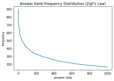
After some searching, I found a public dataset containing nearly every New York Times crossword from 1976 to 2018 (in total some 14,500 puzzles) in JSON format.1 This amounts to ~1.2 million clue-answer pairs with ~100,000 unique words over all the clues and ~250,000 unique answers. For simplicity, we split the dataset 50/50 into train/test based on whether the publication day is even or odd. Some interesting statistics:
| Answer | Occurrences |
|---|---|
AREA | 896 |
ERA | 883 |
ERIE | 819 |
ERE | 750 |
ALOE | 723 |
| Answer type | Example | Occurrence |
|---|---|---|
| English word | SALT | 56.0% |
| English bigram | TOOSALTY | 23.8% |
| English trigram | SALTANDPEPPER | 6.8% |
| other | APEXAM | 13.4% |
Implementation Framework
Our implementation has two main parts: the Guesser and the Solver. The role of the Guesser is to take a clue and the length of the corresponding slot and generate a set of guesses which are reasonable candidates for the slot. The Guesser reports these guesses with an associated confidence score between 0 and 1. The function signature looks something like:
def guess(clue: str, slot_length: int) -> List[Tuple[str, float]]: ...The role of the Solver is to fill in the grid (using the candidates generated by the Guesser) in such a way that maximizes the total confidence. This involves resolving conflicts between intersecting slots. Clearly, a naïve global search over the space of all guesses is infeasible. A weekday 15×15 grid has a bare minimum of 30 slots (usually twice this many) so any uncertainty in the guesser leads to a growth of  in the search space (where
  is the average number of guesses generated per slot).
In reality, it is not as bad as this analysis makes it seem. Due to the arrangement of black cells, each slot usually only intersects a constant number of other slots on average, which makes the dependency graph quite sparse.2 We will use a heuristic approach similar to simulated annealing to generate a solution.
The Guesser
In order to generate guesses for a given clue, our system looks at other clues that it has previously seen, finds those that are most similar, and then makes a guess based off of their corresponding answers. Quantifying semantic similarity between pieces of text is a common problem in NLP. In this case, we first convert each clue into a vector using a technique called TF-IDF. It operates as follows.
- let
 denote our corpus of documents (each clue in the training data is one document)
 - let
 denote the set of terms in our corpus of documents (each unique word is one term)
 - let
 denote the number of time term
  appears in document
Each document is associated with a vector of length  whose components are given by:
![\[\mathrm{tfidf}_d(t) = \mathrm{tf}_d(t) \cdot \mathrm{idf}_d(t)\]](https://russ-stuff.com/wp-content/ql-cache/quicklatex.com-be6dc3e1d59a2e06c6bad029b5540373_l3.png "Rendered by QuickLaTeX.com")
where
![\[\mathrm{tf}_d(t) = \frac{f_d(t)}{\sum_{t' \in T} f_d(t')}\]](https://russ-stuff.com/wp-content/ql-cache/quicklatex.com-e36695e6aea6da1816651e49df5bdc81_l3.png "Rendered by QuickLaTeX.com")
represents the normalized occurrences of in (hence the name “Term Frequency”), and
![\[\mathrm{idf}_d(f) = \log \frac{|D|}{|\{d \in D \mid f_d(t) > 0\}|}\]](https://russ-stuff.com/wp-content/ql-cache/quicklatex.com-b45851e45481c6f0a870250ce02eae15_l3.png "Rendered by QuickLaTeX.com")
is a scaling term that serves to reduce the weight of terms which appear all over the place throughout the corpus (e.g. “the”) (hence the name “Inverse Document Frequency”). The result is that each clue is mapped to a vector that captures the ‘most important’ words in that clue.
The hope is that semantically similar clues are mapped to points that are close to one another in the vector space. The guesser works by first converting the new clue into a vector in the same manner and then finding the 30 clues which have the greatest cosine-similarity score.3 It then looks at the answers associated with these similar clues and computes a confidence score for each one by considering the similarity scores as well as the presence of repeated answers. Finally, it returns the top 5 (or so) most confident guesses. For example:
>>> guess("red fruit", 5)

[('APPLE', 0.961), ('GRAPE', 0.272), ('SUMAC', 0.249), ('MELON', 0.245)]
The Solver
The solver works by keeping track of a confidence value for each cell in the grid. These values range from 0 to 1 and represent how sure we are that the current character is correct. When we write to a cell for the first time, it inherits the confidence of the guess (as determined by the guesser). We iterate over the slots starting with the slots that we are most confident in and working our way down to the less confident guesses. When we encounter a slot that has already been partially filled, we overwrite it if the confidence in our new guess is greater than the average confidence of the cells that would need to be changed.
When a cell is contradicted, it inherits the confidence of the new guess. When a cell is corroborated, it’s confidence is increased according to the following rule:
![\[c \gets 1 - (1 - c)(1 - c')\]](https://russ-stuff.com/wp-content/ql-cache/quicklatex.com-b94e4d26647988ce27cc9a20a096bd2d_l3.png "Rendered by QuickLaTeX.com")
which results from interpreting the old guess confidence  and new guess confidence
  as independent probabilities.
We continue this process until the solver converges on a solution. At this point, if there are still empty cells, we resort to n-gram searching, where we simply attempt to fill in any gaps by searching for sequences of English words that are compatible with the slot. This is accomplished efficiently using regular expressions and a dynamic programming algorithm.
Performance
Despite the simple approach, the performance is respectable. I ran it on the entire test set (which took about 15 hours) keeping track of the portion of cells that were filled in, what portion of those cells were correct, and the product of those two values (which I call the “score”).
- average fill percentage: 93%
- average fill accuracy: 70%
- average score: 65%
One other interesting tidbit is that the performance seems to be correlated with the day-of-the-week. Mondays are designed to be the easiest and Saturdays the hardest (with Sundays somewhere in between). This is reflected in the average scores:
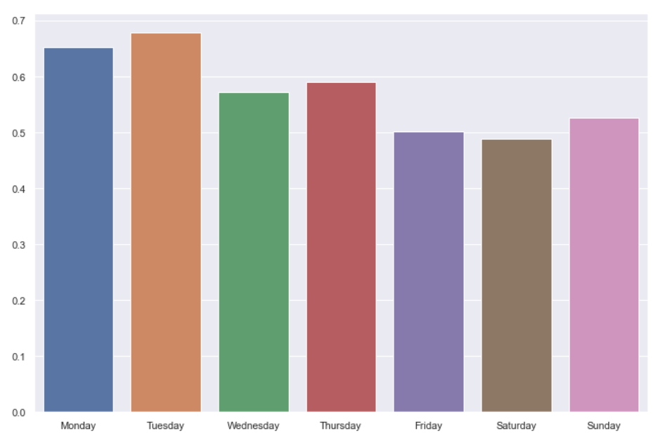
I suppose the take-away here is that harder-for-human can sometimes also mean harder-for-computer 🙂
Link to the repo: https://github.com/rschwa6308/Crossword-Puzzle-Solver
Neat